Chipotle Item Analysis

This is short exploratory walk through of an extract of transaction data (with no customer id but just order id) of orders at Chipotle. Main components are about how are different items priced at this Mexican Grill Cuisine and what are the common add-ons that orders include while a food lover customizes the order.

from collections import Counter  # for generating frequency count using dictionary

import matplotlib.pyplot as plt
import pandas as pd

from wordcloud import (  # for generating word cloud
    STOPWORDS,
    ImageColorGenerator,
    WordCloud,
)

data = pd.read_csv("chipotle.tsv", sep="\t")

Data wrangling

# replace $ and convert item_price to float
data["item_price"] = pd.Series(data["item_price"].str.replace("$", ""), dtype="float")

data.sample(5)

	order_id	quantity	item_name	choice_description	item_price
3264	1306	1	Canned Soft Drink	[Sprite]	1.25
1655	669	1	Chips	NaN	2.15
2022	815	1	Canned Soft Drink	[Diet Coke]	1.25
3306	1325	1	Chips	NaN	2.15
82	36	1	Chicken Burrito	[Fresh Tomato Salsa, [Rice, Black Beans, Chees...	8.75

Summary stats

print(
    "There are {} observations and {} features in this dataset. They are {}. \n".format(
        data.shape[0], data.shape[1], ", ".join(list(data.columns))
    )
)

print(
    "There are {} different items in this dataset such as {}... \n".format(
        len(data.item_name.unique()), ", ".join(data.item_name.unique()[0:5])
    )
)

print(
    "There are {} unique orders in this dataset. \n".format(
        len(data["order_id"].unique())
    )
)

print(
    "The total revenue generated from the orders within is about ${} USD. \n".format(
        round(sum(data["item_price"]), 0)
    )
)

There are 4622 observations and 5 features in this dataset. They are order_id, quantity, item_name, choice_description, item_price. 

There are 50 different items in this dataset such as Chips and Fresh Tomato Salsa, Izze, Nantucket Nectar, Chips and Tomatillo-Green Chili Salsa, Chicken Bowl... 

There are 1834 unique orders in this dataset. 

The total revenue generated from the orders within is about $34500.0 USD. 

Avg. Price across all orders

by_order = pd.DataFrame(data.groupby(by="order_id").agg("sum").reset_index())
by_order = by_order.rename(columns={"item_price": "order_amount"})

# avg. order price
print(
    "The avg. order price is $",
    round(sum(by_order["order_amount"]) / len(by_order["order_amount"]), 2),
)

The avg. order price is $ 18.81

Avg. price paid by each order

by_order = pd.DataFrame(
    data.groupby(by="order_id")
    .agg({"item_price": "mean", "item_name": "count"})
    .reset_index()
)
by_order = by_order.rename(
    columns={"item_price": "avg_order_amount", "item_name": "num_items"}
)

# Distribution of avg. order amount across all orders
plt.hist(by_order["avg_order_amount"])
plt.xlabel("Avg. Order Amount in USD")
plt.ylabel("Frequency count")
plt.show()

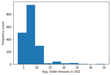
It’s reasonable to see most of the orders paying under $15 for a fast-casual market player. Customers tend to buy shorter orders more often than ordering in bulk which is a rarity.

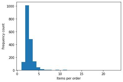
Distribution of items per order

plt.hist(by_order["num_items"], bins=25)
plt.xlabel("Items per order")
plt.ylabel("Frequency count")
plt.show()

by_item_numbers = (
    by_order.groupby(by="num_items").agg({"order_id": "count"}).reset_index()
)
by_item_numbers = by_item_numbers.rename(columns={"order_id": "num_orders"})
by_item_numbers

	num_items	num_orders
0	1	128
1	2	1012
2	3	484
3	4	134
4	5	44
5	6	14
6	7	4
7	8	5
8	9	2
9	10	1
10	11	3
11	12	1
12	14	1
13	23	1

Close to about 55% of the orders are 2-item orders analogous to people ordering a main item with either a side or a beverage. Appently, the next in number of orders is those with 3 items (main item + side + beverage).

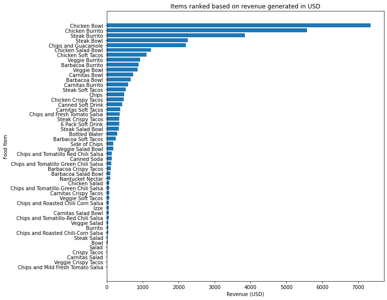
Avg. prices per item ordered

As the each item ordered in any order is customized based on choice description, let’s see what are the avg. prices per item ordered.

# avg. price per item ordered
by_item = pd.DataFrame(
    data.groupby(by="item_name")
    .agg({"item_price": "mean", "order_id": "count"})
    .reset_index()
)
by_item = by_item.rename(
    columns={"item_price": "avg_price_paid", "order_id": "times_ordered"}
)

by_item["revenue"] = by_item["avg_price_paid"] * by_item["times_ordered"]

plt.figure(figsize=(10, 10))
by_item = by_item.sort_values(by="revenue", ascending=True)
plt.barh(by_item["item_name"], by_item["revenue"])
plt.xlabel("Revenue (USD)")
plt.ylabel("Food Item")
plt.title("Items ranked based on revenue generated in USD")
plt.show()

By most ordered

# Top 5items by 'times_ordered'
by_item.sort_values(by=["times_ordered"], ascending=False)[:10]

	item_name	avg_price_paid	times_ordered	revenue
17	Chicken Bowl	10.113953	726	7342.73
18	Chicken Burrito	10.082857	553	5575.82
25	Chips and Guacamole	4.595073	479	2201.04
39	Steak Burrito	10.465842	368	3851.43
10	Canned Soft Drink	1.457641	301	438.75
38	Steak Bowl	10.711801	211	2260.19
23	Chips	2.342844	211	494.34
6	Bottled Water	1.867654	162	302.56
22	Chicken Soft Tacos	9.635565	115	1108.09
21	Chicken Salad Bowl	11.170455	110	1228.75

• Canned Soft Drink is the most ordered beverage.

By revenue

by_item.sort_values(by=["revenue"], ascending=False)[:10]

	item_name	avg_price_paid	times_ordered	revenue
17	Chicken Bowl	10.113953	726	7342.73
18	Chicken Burrito	10.082857	553	5575.82
39	Steak Burrito	10.465842	368	3851.43
38	Steak Bowl	10.711801	211	2260.19
25	Chips and Guacamole	4.595073	479	2201.04
21	Chicken Salad Bowl	11.170455	110	1228.75
22	Chicken Soft Tacos	9.635565	115	1108.09
45	Veggie Burrito	9.839684	95	934.77
2	Barbacoa Burrito	9.832418	91	894.75
44	Veggie Bowl	10.211647	85	867.99

• Chicken Bowl, Chicken Burrito, Steak Burrito, Steak Bowl get us the most revenue.
• Chips and Guacamole is the most ordered as well as revenue-generating sides

List of all the items where customization was possible

df_without_na = pd.DataFrame(data.dropna())

# Items for choice_description is possible
pd.Series(df_without_na["item_name"].unique())

0                      Izze
1          Nantucket Nectar
2              Chicken Bowl
3             Steak Burrito
4          Steak Soft Tacos
5      Chicken Crispy Tacos
6        Chicken Soft Tacos
7           Chicken Burrito
8               Canned Soda
9          Barbacoa Burrito
10         Carnitas Burrito
11            Carnitas Bowl
12            Barbacoa Bowl
13       Chicken Salad Bowl
14               Steak Bowl
15      Barbacoa Soft Tacos
16           Veggie Burrito
17              Veggie Bowl
18       Steak Crispy Tacos
19    Barbacoa Crispy Tacos
20        Veggie Salad Bowl
21      Carnitas Soft Tacos
22            Chicken Salad
23        Canned Soft Drink
24         Steak Salad Bowl
25        6 Pack Soft Drink
26                     Bowl
27                  Burrito
28             Crispy Tacos
29    Carnitas Crispy Tacos
30              Steak Salad
31        Veggie Soft Tacos
32      Carnitas Salad Bowl
33      Barbacoa Salad Bowl
34                    Salad
35      Veggie Crispy Tacos
36             Veggie Salad
37           Carnitas Salad
dtype: object

# Calling list_to_string function
%run list_to_string.py

This is a neat way of getting a paricular task done by calling a function added in a .py file. It makes code easy to read for future reference and our team members.

# data transformation to string without any [] in the choice_description column
df_without_na["choice_description"] = df_without_na["choice_description"].apply(
    list_to_string
)

text = ", ".join(cd for cd in df_without_na.choice_description)
print("There are {} choice additions in the choice descriptions of all the items ordered.".format(len(text)))
my_list = text.split(", ")
word_count_dict = Counter(my_list)

There are 210889 choice additions in the choice descriptions of all the items ordered.

What goes in the add-ons/choice description mostly?

wordcloud = WordCloud(
    max_words = 100, background_color="white", width=1600, height=1200, scale=1.5
).generate_from_frequencies(word_count_dict)

# Display the generated image
plt.figure(figsize=(10, 15))
plt.imshow(wordcloud, interpolation="bilinear")
plt.axis("off")
plt.show()

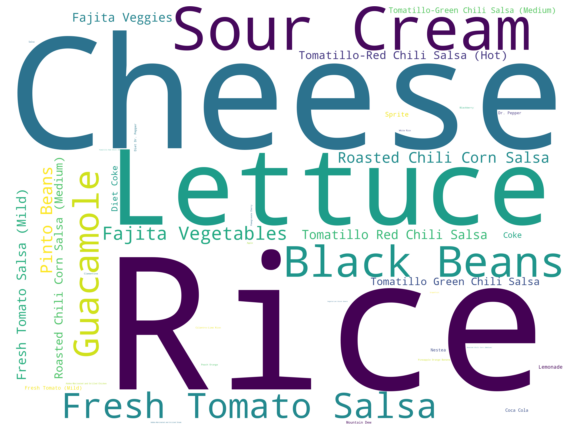
Just by looking at the wordcloud, a couple of insights are clearly visible:

• In all the orders pertaining to this dataset, a bowl or a burrito has Rice, Lettuce, Cheese, Sour cream as add-ons. While this maybe trivial to some of you, especially those from the Mexican descent, for someone who don’t know anything about the Mexican cuisine like me, this is valuable information to form hypothesis. This applies to any data set one works on. In some cases, we as data analysts/scientists are pre-informed but in some cases, data itself tells us the new information we do not know till that point. It’s about asking the right questions.
• Among Salsa’s, Fresh Tomato Salsa looks to be the top added add-on and then Roasted Chili Corn Salsa.
• As beans are common in Mexican food, both Black and Pinto beans are visible in the top 100 add-ons. But as a matter of fact, Black beans has lower carbs than Pinto beans which could be a reason as all the food lovers like us in this data are preferring Black Beans.

What are the items which doesn’t have any choice_description (no customization)?

set(data["item_name"].unique()) - set(df_without_na["item_name"].unique())

{'Bottled Water',
 'Chips',
 'Chips and Fresh Tomato Salsa',
 'Chips and Guacamole',
 'Chips and Mild Fresh Tomato Salsa',
 'Chips and Roasted Chili Corn Salsa',
 'Chips and Roasted Chili-Corn Salsa',
 'Chips and Tomatillo Green Chili Salsa',
 'Chips and Tomatillo Red Chili Salsa',
 'Chips and Tomatillo-Green Chili Salsa',
 'Chips and Tomatillo-Red Chili Salsa',
 'Side of Chips'}

A good check that the sides are mostly not customizable - data sanity check. It’s good to have these sanity checks once in a while all through the data analysis and modelling to ensure reliable results. But that’s not the end as there can be variation depending on the region, season, etc. That’s where as a data analyst/scientist, one has to use communicate with a team member or someone in a senior role to clarify whether all the listed elements are not customizable. More generally, it’s important to understand the holistic view of what the business is trying to achieve. Ultimately, data tells a story partially, to make it whole, business knowledge (as simple as the above example) and team play is necessary.

This brings to the end of this simple walk-through (fully accessible via this repo) and my plan from here on is to extend this analysis for a market basket analysis or to recommend what can a customer add as an add-on for a future order.

Off to pondering whether this data is sufficient to do what struck me. If you have any ideas or loves to try different food cuisines, ping me - we can discuss about food or plan to implement the ideas for a great customer experience…

Trivia

What is the avg. number of orders in a week at Chipotle (any location)?

Let’s guesstimate…

Equation: No. of restaurants of Chipotle x No. of weeks in a year (wk) x No. of orders per week (orders/wk) x Revenue per order (USD/orders) = Total annual revenue (USD). Check if the units are balanced on both sides.

We get the Revenue per order from the above dataset. (remember this is an avg. figure) = $(34500/1834) USD. The other data points like revenue and no. of locations are openly available.

Assumptions

Inevitably, valid assumptions are key to calculating estimates:

• A core assumption to this particular calculation is - the revenue generated in this data set is only for a single location/restaurant.
• Chipotle’s annual revenue amounts to what it is just because of food orders
• The total revenue amounts to both in-store and online sales.

No. of orders per week = 6B (USD) / (2500 * 52 * No. of orders per week * (34500/1834))

Turns out to be ~ 2453 orders per week.

This is only an approximation based on the assumptions made. Actual numbers might vary a lot depending on the location, season, things like COVID-19. There might also be other sources of revenue other than food ordering which hasn’t been accounted for in this calculation.